State Space Models with a Common Stochastic Variance
Introduction
In the paper `State Space Models with a Common Stochastic Variance' by
, an estimation method is presented for combinations
of the stochastic volatility model
and the general linear state space model
with a common fixed variance
s2, that is
where y
t is a p ×1 vector of observations, c
t is a p×1 vector of fixed effects (possibly containing regressor
variables),
at is a m
a ×1
vector of unobserved states and
et is a r×1 vector of disturbances. The system matrices Z
t, T
t,
G
t and H
t are assumed to be fixed for all time points
t=1,
¼,n. Unknown elements of the system matrices will be treated
as parameters to be estimated by the method of maximum likelihood.
The two models are easily combined by changing the common fixed variance
s2 in (
2) with the time varying variance of
(
1).
This page presents the programs used in obtaining the results.
Programs and installation
The package
ssfsv4.zip contains the necessary files and data for
estimating models in state space using simulated maximum likelihood.
Unpack the file to a directory of your choice. For graphical output,
either the original
OxDraw routines of
Ox 7 can be
used, or alternatively one can install
GnuDraw.
The programs depend on the extended version of
SsfPack, of
Siem Jan Koopman.
The installation file contains a
readme.txt
explaining the contents of the package. Most instructive is the program
ssfsvest5.ox which estimates an SV model based on
settings in
simox.dec.
Some usage hints
The package declares an object of type
SSFSV(), deriving from the
Ox
Modelbase
class. Using the standard Modelbase routines, a dataset should be set
up, selecting the exogenous variables as usual.
The model is specified using a call similar to
Ssfsv.ChooseModel(<CMP_LEVEL, .05, 0, 0;
                   CMP_SEAS_DUMMY, .025, 12, 0;
                   CMP_IRREG, .15, 0, 0;
                   CMP_SV, .2, 0, .95>);
which would specify a local level model with seasonal effects, and a
common stochastic variance component with, initially, standard deviation
sx = 0.2 and persistence
f = 0.95.
After setting up the model, estimation is done with the usual call to
Ssfsv.Estimate();
Note that estimation can be time consuming, especially if the number of
importance samples is large.
Selected results
With the above settings in the file
declinfl/infl_llssv.dec copied over
simox.dec, running the program
oxl ssfsvest5
results in Ox output as displayed in
Table
1 below, equal to results in .
Graphical output is created to show the
states estimates as in Figure
1, weights, residual
analysis and much more.
Table 1: Results of optimisation
---- SsfSV ----
The estimation sample is:  1957 (1) - 2001 (9)
The dependent variable is: dLcuur
                  Coefficient     Confidence bounds        Score
s(Lev)              0.0296983  [  0.02042,  0.04319]  <2.423e-07>
s(Seas_dum)         0.0370710  [  0.02506,  0.05484]  <3.642e-07>
s(Irr)               0.139992  [   0.1061,   0.1847]  <1.805e-06>
s(SV)                0.216399  [   0.1467,   0.3192]  <2.384e-06>
phi(SV)              0.963198  [   0.9193,   0.9837]  <-2.103e-06>

log-likelihood     153.137492
no. of observations       537  no. of parameters           5
AIC.T             -296.274984  AIC              -0.551722502
mean(dLcuur)         0.350417  var(dLcuur)         0.0889883
Using maximum likelihood estimation and transformed parameters
with the exact likelihood
  in a time of 25:05.61
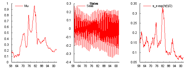
Table 2: State estimates as for the model with common stochastic
variance
Routines in the package
Apart from the normal Modelbase routines, some added functions
provided are
-
#import "include/ssfsv"
ChooseModel(const mStsm);
- mStsm
- in: Matrix to indicate the type of State Space model. Apart from the
standard Ssfpack elements, also components for an SV model, for GARCH or
for ARMA are possible. See the declaration files for examples.
[
Top]
-
#import "include/ssfsv"
ChooseSVRep(const iMaxRep, const iSimSV);
ChooseSVRep(const iMaxRep, const iSimSV, const bApprox);
- iMaxRep
- in: integer, indicating the maximum number of repetitions to use
while searching for the approximating model (default=50, use -1 to keep
old value).
- iSimSV
- in: integer, number of simulations used in the importance sampler
(default=250, use -1 to keep old value).
- bApprox
- in: boolean, indicating if an approximative (but quicker) likelihood
should be used (default=FALSE).
[
Top]
-
#import "include/ssfsv"
ChooseTransform(const bUseTransform);
- bUseTransform
- in: boolean, indicating if a transformation of the parameters should
be used or not (default=TRUE)
[
Top]
-
#import "include/ssfsv"
SetSampleZoom(const iZoom1, const iZoom2);
- iZoom1, iZoom2
- in: integers, indicating indices of first and last observation to
which we zoom in, e.g. when looking at the weight graphs.
[
Top]
-
#import "include/ssfsv"
SSFSVLikelihood(const vP, const adFunc, const avScore, const amHessian);
- vP, adFunc, avScore, amHessian
- See MaxBFGS; this routine provides the likelihood function of the
model
[
Top]
-
#import "include/ssfsv"
GenerateSsf(const vP, asName);
- vP
- in: Vector of parameters of the model
- asName
- in: String, or array of strings, with name of variable, under which
the newly generated data is stored in the database.
[
Top]
-
#import "include/ssfsv"
GetISWeights();
- Return value
- mWgt: 2 x iSim matrix with importance sampler weights.
[
Top]
-
#import "include/ssfsv"
GetConfBounds();
- Return value
- mLU: iP x 2 matrix with the bounds of the (non-symmetric, if
transformed parameters were used) confidence region.
[
Top]
-
#import "include/ssfsv"
SaveGraphics(const sGraphbase);
- sGraphbase
- in: String with the basename for saving graphics; if the empty
string is given, no graphs are saved.
[
Top]
-
#import "include/ssfsv"
TestAuxResiduals(vbSel, vbPlot, const dLimit, const bWrite);
TestCorrelogram();
TestFinal();
TestGoodFit();
TestGraphics(vbPlot, const bFilt, const iaLog, const iNLSeas);
TestISWeightGraphs(dQ);
TestNormality(const vRes, const sName);
TestResiduals(vbPlot, const iLag, const bWrite);
TestParameterGraphs();
TestSummary(const bShow);
TestWeightGraphs(const vP, iW);
- Set of testing routines, see actual programs for their usage.
[
Top]
Bibliography
Koopman, S. J. and Bos, C. S. 2004
, `State space models with a common stochastic variance', Journal of
Business and Economic Statistics 22(3), 346-357. [ http ]
File translated from
TEX
by
TTH,
version 3.77.
On 22 Mar 2011, 16:09.